Bulletin – December 2018 Australian Economy Business Concentration and Mark-ups in the Retail Trade Sector

The Australian product market has undergone significant structural change over recent decades. Changes include the emergence of highly integrated global supply chains, the growth of ‘big box’ retailers, and the rapid rise of e-commerce and price comparison technology (Productivity Commission 2011). These structural changes have affected the nature of competition and the extent of market power among Australian businesses, particularly those operating in the retail trade sector (D'Arcy, Norman and Shan 2012). This, in turn, is likely to have affected the allocation of resources and consumer outcomes; firms with market power can set their prices above marginal cost (the cost of producing one more unit of output) and produce less output, which reduces consumer welfare.

Competition and market power have normally been considered the domain of microeconomics, but macroeconomists have become increasingly interested in these topics (De Loecker and Eeckhout 2017; Hall 2018). This is partly because the level of competition in the economy can affect key macroeconomic variables and the relationships between them. Consumer price inflation in Australia has been unusually weak in recent years, despite low unemployment and above-trend economic growth. Greater competition in the retail trade sector may have affected not only the level of price inflation but also the sensitivity of inflation to changes in economic conditions (Haldane 2018). The extent of market power can also affect incentives for firms to innovate, which in turn affects business investment, productivity and potential growth in the economy (De Loecker and Eeckhout 2017; Gutiérrez and Philippon 2017).

In this article we explore trends in competition among Australian businesses using two key indicators: the share of sales accounted for by the largest firms in an industry (or business concentration); and the ratio of prices to marginal cost (or mark-ups). We find that business concentration has risen in recent years, most notably in the retail trade sector. At the same time, mark-ups in the retail trade sector have declined, after increasing over the 2000s.

Taken together, these findings may appear puzzling – how can a sector become increasingly dominated by a few large players and yet be more price competitive? Microeconomic theory has shown that business concentration is not the same thing as competition. An industry can be very concentrated and highly competitive. An industry can be very dispersed and uncompetitive too. The level of competition in an industry partly depends on how many businesses there are and how big they are. But it also depends on other factors, such as how easily new firms can enter the industry, and whether consumers can easily switch between different firms' products.

The trends in business concentration and mark-ups in retail trade can be reconciled by recognising that competitive dynamics in the sector are not well captured by concentration measures. For example, the entry of a large player in an industry that has two big incumbent firms and many small businesses is likely to lead to greater market concentration, but could represent more competition for the large incumbents. In either case, the entry of this large market player is likely to be seen by the small businesses as increased competition. We explore some of these issues in this article.

How Should We Measure Business Competition?

Business competition is hard to observe directly so we take two complementary approaches to measure it. First, we observe business concentration – the share of output accounted for by the largest firms in an industry – which is a common measure of competition. Second, we estimate firm-level mark-ups – the ratio of price to marginal cost – which is a more theoretically appealing measure of business competition.

In this article, our key indicator of business concentration is the top four concentration ratio (CR4) – the combined market share of the top four largest producing firms in each four-digit Australian and New Zealand Standard Industrial Classification (ANZSIC) industry and year.^[1] The market share of each business is estimated based on gross output, or total sales (less GST). This is sourced from Business Activity Statements (BAS) that almost every Australian business must submit to the Australian Tax Office. These data are available in the Business Longitudinal Analysis Data Environment (BLADE), which provides unit record data for the population of employing Australian businesses over the period from 2001/02 to 2014/15.

We can also infer competition from estimates of mark-ups, which we construct for each firm using the same tax data. These mark-ups measure the degree to which prices exceed marginal costs. In theory, firms set their price as a mark-up over marginal cost, and the size of the mark-up is directly linked to the firm's market power. As such, mark-ups represent a theoretically sound measure of that market power.

In measuring competition, there are a few data issues in the BLADE dataset to highlight. A ‘firm’ in BLADE is any entity with an Australian Business Number (ABN) that has to submit a BAS. This means that a retail conglomerate, such as Wesfarmers, will appear multiple times in the dataset under, for example, hardware (Bunnings) and department stores (Kmart and Target). On Australian Bureau of Statistics (ABS) definitions, Wesfarmers is known as an ‘enterprise group’ and Bunnings, Kmart and Target are ‘type of activity units’. In this article we do not have access to information about each firm's enterprise group so we cannot identify the effect of conglomerates on overall competition within the retail trade sector.^[2]

How Has Business Concentration Changed across Industries and over Time?

Before we focus on the retail trade sector, it is worth considering what has happened to business concentration across all Australian industries. Applying a rule of thumb that a market is concentrated if the largest four firms control one-third (or more) of total output, over half of the industries in Australia are concentrated. In 2014/15, the top four largest firms in each industry accounted for about 42 per cent of total industry output on average (and 37 per cent in the median industry). These estimates are very similar to that in Leigh and Triggs (2016) who measure business concentration in Australia in 2016 using a dataset covering public and private companies.

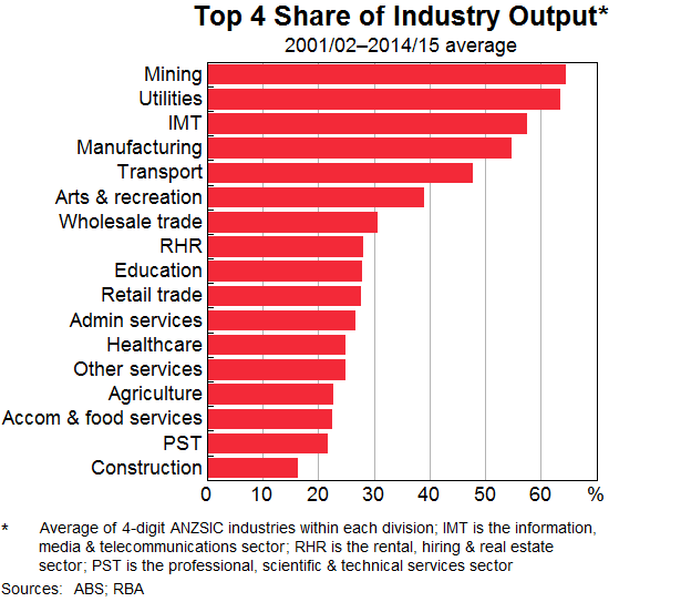
The degree of business concentration varies a lot by industry. There are quite a few industries that are dominated by a small number of firms, with the top four firms account for basically all output. On the other hand, in a relatively large share of industries the largest four firms account for less than half of total industry output. The most concentrated industries tend to be in the mining, utilities, and information media & telecommunication sectors (Graph 1). The manufacturing sector also features prominently; it is likely that only the biggest firms have survived the increase in import competition over recent decades. At th other end of the spectrum, the least concentrated industries are typically in sectors such as construction, accommodation & food services, and professional, scientific & technical services. Overall, the results are similar to previous Australian studies (e.g. Leigh and Triggs (2016))

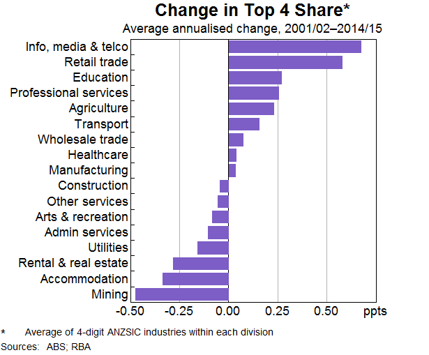
Business concentration has increased steadily since the start of this century. Overall, about 78 per cent of Australian four-digit ANZSIC industries are estimated to have recorded an increase in concentration between 2001/02 and 2014/15. The industries that became more concentrated are typically in services sectors, including information, media & telecommunications, retail trade, and education services (Graph 2). The industries that became less concentrated over this time are generally in the mining, accommodation & food services, and rental, hiring and real estate services.

What Has Happened to Concentration in the Retail Trade Sector?

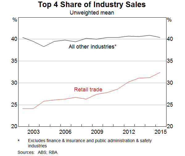
The retail trade sector accounts for much of the overall increase in business concentration in Australia (Graph 3). On average across all retail industries, the top four largest firms increased their share of industry sales from about 24 per cent to 32 per cent between 2001/02 and 2014/15.

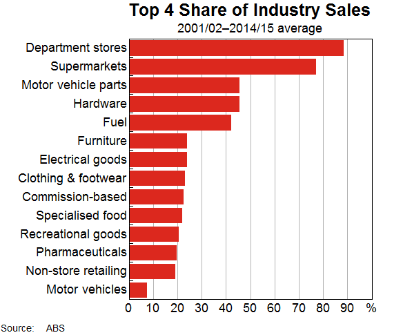
Digging deeper, the parts of the retail trade sector that are most concentrated include department stores and supermarkets (Graph 4). The retail trade industries that are less concentrated include motor vehicle retailing and non-store retailing.

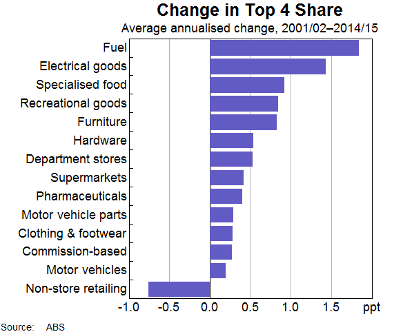
The increase in concentration within the retail sector has been fairly broad based across industries (Graph 5). The largest increases in concentration have occurred in fuel and electrical goods retailing. Non-store retailing was one of the few retail industries in which concentration is estimated to have declined.

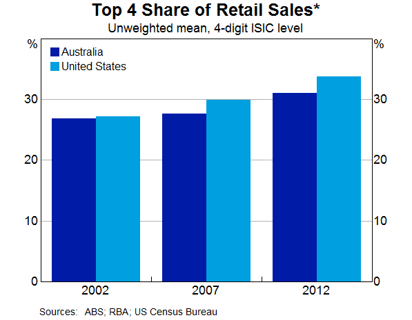
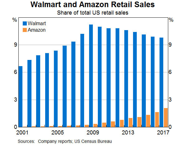
The increase in concentration in the Australian retail sector over recent decades is similar to that observed in the United States (Graph 6).^[3] This may suggest that common forces are at play. In the United States, a couple of large players account for much of the increase in market concentration in the retail trade sector. For instance, listed company annual report data indicate that the retail giant Walmart accounted for a large share of the increase in US retail trade concentration during the 2000s (Graph 7). More recently, the online retailer Amazon has been rapidly gaining market share.

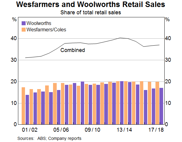
Undertaking a similar analysis for Australia, the combined market share of Wesfarmers (including Coles) and Woolworths increased from around 30 per cent of total retail trade in 2001 to peak at about 40 per cent in 2013 (Graph 8). On top of this, concentration has tended to increase in retail industries where the two large retail conglomerates have become more dominant. This suggests that these two conglomerates could explain a large fraction of the estimated rise in business concentration that is apparent in the BLADE data. However, as highlighted earlier, we cannot directly test this idea because we cannot identify these retail conglomerates in the data. By the same logic, the estimates of business concentration will not be affected by the sale of Coles by Wesfarmers in November 2018 given that we cannot directly identify the supermarket in the data.

What Has Happened to Mark-ups in the Retail Trade Sector?

As an alternative indicator of retail competition, we estimate firm-level mark-ups using the method proposed by De Loecker and Warzynski (2012). This approach relies on the fact that, if a firm is minimising its costs, its mark-up will be equal to the ratio of its elasticity of output with respect to labour (i.e. how much additional output is produced if the firm employs extra labour) over the share of revenue it pays out in wages.^[4] While we can directly observe the share of revenue paid out as wages, we need to estimate the elasticity using data on the firm's inputs and output. This is an indirect way of measuring the degree of competition because it measures the outcome of competition. It is expressed as the ratio of the price to the marginal cost, though these two components cannot be separately identified by this method. So a value of 1.5 indicates that the price is 50 per cent higher than the marginal cost.

We present two aggregate measures of retail mark-ups, which we refer to as the ‘unweighted’ and ‘sales-weighted’ average mark-ups, each of which provides different information. The unweighted average provides information on the mark-up of the ‘typical’ retailer. The sales-weighted average provides information on the average mark-up ‘paid’ by consumers, so it should be the measure most relevant to consumer welfare.

The weighted measure is generally higher than the unweighted measure, indicating that large retailers have higher mark-ups (Graph 9). This is consistent with the large retailers having more market power. The gap between the weighted and unweighted estimates has grown over time. Given it is a sales-weighted average of the individual firm mark-ups, this could indicate either that the large retailers have gained market share, or that they have increased their mark-ups, or both. We find that the growing gap is mainly due to the large retailers gaining market share based on the Melitz and Polanec (2015) accounting decomposition.^[5] This is consistent with the trends in business concentration.

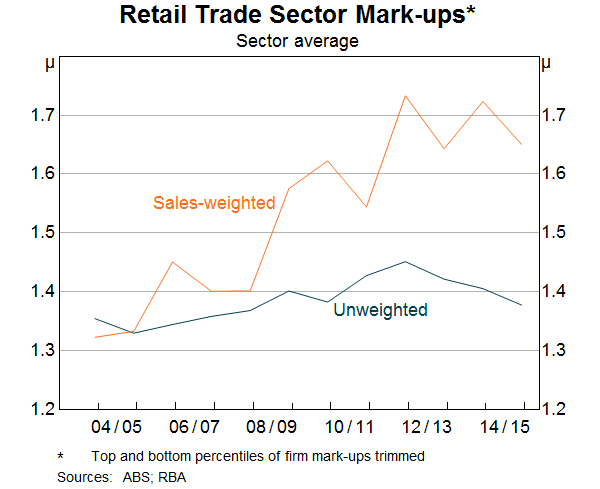
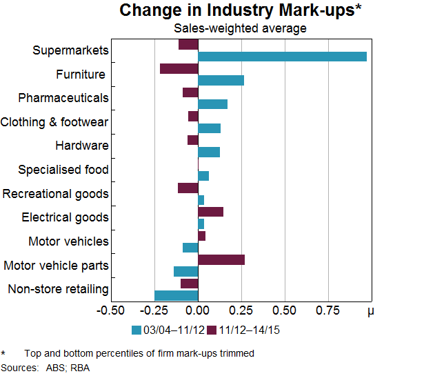
Also consistent with the increase in retail concentration, aggregate retail mark-ups increased over the mid 2000s, indicating decreasing competitive pressures. Moreover, as with concentration, the increase was broad based across most industries over the sample period (Graph 10). However, unlike the measures of concentration, mark-ups peaked in 2012 and have generally fallen since then. This finding is consistent with reports of increased retail competition in recent years.

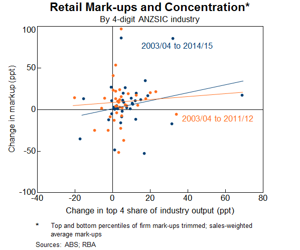
Estimates of business concentration and mark-ups tell us what has happened to competition, but not why. As such, it is informative to explore what factors are associated with the changes in mark-ups and concentration. For example, there is a positive correlation between our estimates of concentration and mark-ups; retail industries that experienced larger increase in concentration also tended to experience larger increases in mark-ups (Graph 11).^[6] Industry-level regressions support the graphical findings. So the number and size of firms in an industry does appear to be important in determining the level of competition.

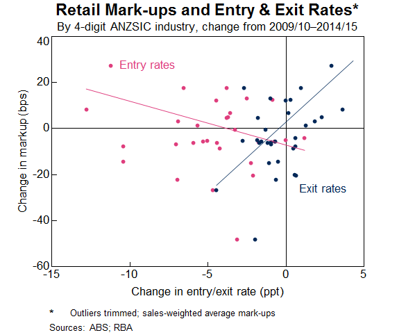
But there is also evidence that barriers to entry and exit are important determinants of retail competition. Based on published ABS estimates of business entry and exit, it is evident that the retail industries with larger falls in entry rates have experienced larger increases in mark-ups, on average (Graph 12).^[7] Also, industries with increasing exit rates have seen larger increases in mark-ups. This is consistent with surviving retailers maintaining high mark-ups in the face of lower competition. It may also reflect small retailers (with lower mark-ups) being squeezed out by larger retailers.

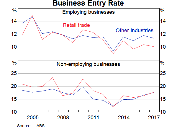
Looking at changes over time, the entry rate of both employing and non-employing retailers steadily fell over the 2000s (Graph 13). But, more recently, the entry rate of employing retailers has been relatively flat while the entry rate of non-employing retailers has picked up slightly. This may suggest that barriers to entering the retail trade sector have been lower in recent times, which would be consistent with a more competitive retail environment. But the recent trends in retail entry rates have been closely matched by entry rates for other industries, which suggests that an economy-wide factor is driving this change in business dynamism, rather than an increase in retail sector competition.

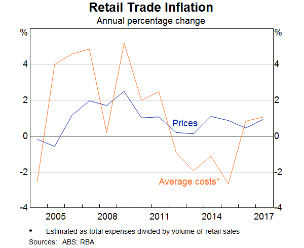
Finally, we examine the link between mark-ups and retail price inflation. It is somewhat puzzling that retail price inflation has been so weak in recent years while the sales-weighted measure of mark-ups has flattened out, rather than declined. The combination of relatively stable mark-ups and weak retail price inflation could reflect that retailers respond to the heightened competition by lowering marginal costs. While we cannot observe marginal costs directly, we can infer what has happened to average costs, which should follow similar trends over time. There is clear evidence of a decline in the growth of average costs through much of the 2010s (Graph 14). This is consistent with anecdotal evidence provided by retailers through the Bank's business liaison program.

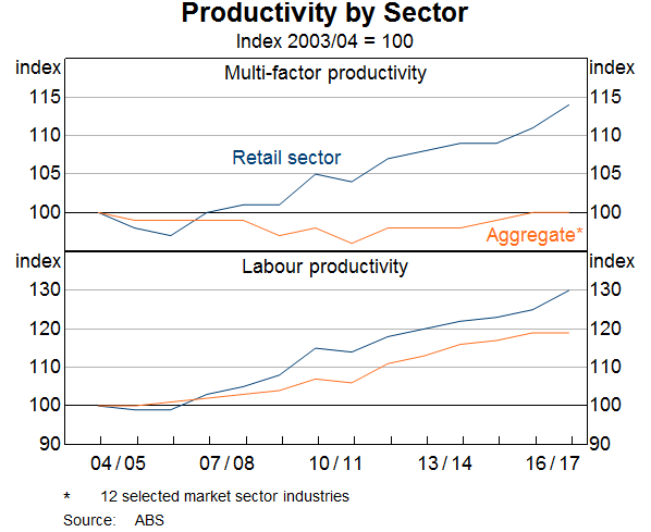
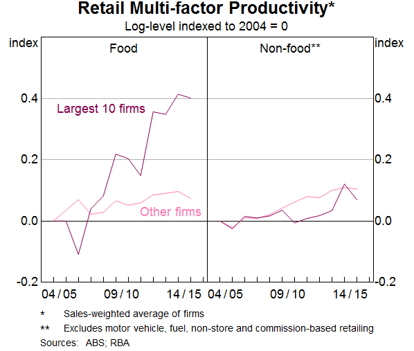
These lower costs might reflect retailers responding to heightened competition by lifting productivity. There is evidence that retailers have increased their productivity relative to other sectors of the economy over the past decade. ABS estimates indicate that, since 2003/04, multi-factor productivity in the retail sector has risen by around 15 per cent, while it has not grown at all for the economy as a whole (Graph 15). Firm-level evidence suggests that, at least in food retailing, it is the largest firms that have had the largest increases in productivity (Graph 16).^[8]

Conclusion

The average Australian industry has become more concentrated since the start of this century. This increase in concentration has been most pronounced in the retail trade sector, particularly in recent years. Estimates of retail mark-ups suggest that retail prices rose relative to marginal costs over the 2000s but have declined in recent years. We also find that these competition indicators are correlated with the entry and exit rates of retailers, suggesting that barriers to competition may be important. Overall, the retail trade sector appears to have become more competitive in recent times, most notably among the largest retailers, following a period of declining competition through the 2000s.

Appendix

The method outlined in De Loecker and Warzynski (2012) relies on the assumption that firms are cost minimisers and that labour is fully flexible, but does not require any assumptions about the specific price-setting mechanisms employed by firms. It exploits the fact that, if a firm is a cost minimiser, its mark-up will be proportional to the labour share of revenue (wages divided by revenue). The intuition behind this is as follows. In theory, a perfectly competitive firm sets its price equal to its marginal cost, and this implies that the firm's labour share of revenue is equal to its elasticity of output with respect to labour (i.e. how much additional output is produced if the firm employs extra labour). In contrast, a firm with market power sets a higher price, which includes a mark-up over the marginal cost. As they set a higher price, the firm will tend to produce and sell fewer goods, and so will employ less labour. But, as the firm sells the goods at a higher price, revenue does not decline by as much as their wage payments, so the labour share declines.

More formally, De Loecker and Warzynski (2012) show that for a cost minimising firm, the optimal mark-up, μ_i, will be proportional to: the output elasticity for a variable input, such as labour, ∝_l; and the share of expenditure on that input, relative to total sales, $\frac{W_i{L}_i}{P_i{Y}_i}$ :

$${\mu }_i={\propto }_l/\left(\frac{W_i{L}_i}{P_i{Y}_i}\right)$$

This is a general result that holds for various different competitive structures and price-setting mechanisms (see Online Appendix to De Loecker and Warzynski (2012)).

Firms' total sales and expenditures on inputs are readily available in BLADE. However, estimates of the output elasticity are not. De Loecker and Warzynski (2012) suggest taking these elasticities from production functions, which can be estimated using various methods proposed in the literature. Below is a brief overview of the approach that we take.

Consider the following Cobb Douglas production function for gross-value added (GVA) expressed in logs:^[9]

Equation 1 $$gv{a}_{i,t}={\propto }_l{l}_{i,t}+{\propto }_k{k}_{i,t}+{\omega }_{i,t}+e_{i,t}$$

where $l_{i,t}$ and $k_{i,t}$ the (logged) labour and capital inputs of firm i at time t, ${\omega }_{i,t}$ is the firm's productivity, and $e_{i,t}$ is an i.i.d. shock, such as a measurement error.

This equation cannot be estimated by ordinary least squares (OLS), as firms' choices of inputs, particularly variable inputs, will be correlated with the unobserved productivity term, ${\omega }_{i,t}$ , regarding which we assume the firm has some information.

Following Olley and Pakes (1996), the standard approach taken in the literature is to use some proxy in place of the ${\omega }_{i,t}$ term. We use a measure of materials inputs, $m_{i,t}$ , as our proxy. Assuming that materials are monotonically increasing in productivity, conditional on capital and some other factors that could affect the choice of inputs (such as wages), $z_{i,t}$ , then:

Equation 2 $$m_{i,t}=h_t\left(k_{i,t},{\omega }_{i,t},z_{i,t}\right)$$

and by monotonicity:

Equation 3 $${\omega }_{i,t}=g_t\left(k_{i,t},m_{i,t},z_{i,t}\right)$$

Substituting this into the production function:

Equation 4 $$gv{a}_{i,t}={\propto }_l{l}_{i,t}+{\propto }_k{k}_{i,t}+g_t\left(k_{i,t},m_{i,t},z_{i,t}\right)+e_{i,t}$$

Equation 5 $$gv{a}_{i,t}={\propto }_l{l}_{i,t}+{\varphi }_t\left(k_{i,t},m_{i,t},z_{i,t}\right)+e_{i,t}$$

Assuming that labour is fully flexible, we could estimate Equation 5 using a polynomial of some order in place of the unknown function ${\varphi }_t$ . However, to avoid issues related to functional dependence (essentially non linear multicolinearity) identified by Ackerberg, Caves and Frazer (2015), we instead forgo recovering in ${\propto }_l$ the first step.

Instead, we take the production function to be:

Equation 5a $$gv{a}_{i,t}={\varphi }_t\left(l_{i,t},k_{i,t},m_{i,t},z_{i,t}\right)+e_{i,t}$$

While we know that ${\varphi }_t$ is a function of $l_{i,t},k_{i,t},m_{i,t}$ and $z_{i,t}$ , we don't know the form of this function. As such we recover an estimate of ${\widehat{\varphi }}_t$ by regressing $gv{a}_{i,t}$ on a third-order polynomial in $l_{i,t},k_{i,t},m_{i,t}$ and $z_{i,t}$ . The idea is that this polynomial should be flexible enough to approximate the unknown function.

Combining Equations 1 and 5a, we know that:

Equation 6 $${\omega }_{i,t}={\widehat{\varphi }}_t-{\propto }_l{l}_{i,t}+{\propto }_k{k}_{i,t}$$

While we don't actually observe ${\omega }_{i,t}$ , for any candidate set of $\alpha$ we could calculate:

Equation 7 $${\omega }_{i,t}\left(\alpha \right)={\widehat{\varphi }}_t-{\propto }_l{l}_{i,t}+{\propto }_k{k}_{i,t}$$

We now need some way of assessing different sets of candidate $\alpha$ . To start, we further assume that productivity follows Markov process such that:

Equation 8 $${\omega }_{i,t}=r_t\left({\omega }_{i,t-1}\right)+{\xi }_{i,t}$$

where ${\xi }_{i,t}$ is an i.i.d. productivity shock. That is, knowing the productivity level two or more periods ago would do nothing to help us forecast productivity, conditional on knowing last period's productivity.

Similar to above, we do not know the form of the function $r_t$ . But we can approximate it using a third-order polynomial in ${\omega }_{i,t-1}$ . So, using Equation 7 we know that for any candidate set of $\alpha$ , we can obtain ${\xi }_{i,t}\left(\alpha \right)$ by regressing ${\omega }_{i,t}\left(\alpha \right)$ on a third-order polynomial in ${\omega }_{i,t-1}\left(\alpha \right)$ .

This, along with a few further assumptions, will help us to assess different candidate $\alpha$ . In particular, we assume that it takes some time to plan and make investments, and therefore that the fixed factor $k_{i,t}$ cannot be adjusted in response to unexpected changes in productivity, ${\xi }_{i,t}$ . As such, the two should be uncorrelated. Meanwhile, while the flexible factor labour, $l_{i,t}$ , could be adjusted in response to the shock, labour in the previous period, $l_{i,t-1}$ , can't be adjusted. Therefore it too should be uncorrelated with the unexpected changes in productivity. As such, we want to pick $\alpha$ such that $k_{i,t}$ and the estimated of ${\xi }_{i,t}$ are uncorrelated, and such that $l_{i,t-1}$ and the estimated ${\xi }_{i,t}$ are uncorrelated.

To do this, we use the Generalised Method of Moments (GMM) approach. In particular, we set the above two conditions up as a set of moment restrictions:

Equation 9 $$E\left({\xi }_{i,t}\left(\alpha \right)\left(\begin{array}{c}\begin{array}{c}{l}_{i,t-1}\\ k_{i,t}\end{array}\end{array}\right)\right)=0$$

We then solve this system (i.e. minimise the correlations) using numerical techniques.

Our measure of labour inputs is full-time equivalent employees, while our measure of capital stock is the firm's non-current assets, derived from firms' Business Income Tax returns.^[10] We use the capital stock as at the end of the previous year to make the assumption that the capital stock cannot be adjusted in response to unexpected productivity changes more believable, and to reflect the fact that we have no information on when during the year additional capital becomes usable. Materials are measured as non-capital purchases from the Business Activity Statement (BAS), while value added is constructed as sales from the BAS, less materials. Value added, capital and materials are deflated using retail sector price deflators.

We estimate the models at the four-digit ANZSIC industry level to account for differences between, for example, supermarkets and clothing stores. Any industry with less than 50 firms was removed due to confidentiality concerns and to ensure we have a large enough sample for estimation. This resulted in us dropping the Department Store industry.

As a robustness test, we tried accounting for firm failure by including an estimate of firm probability of failure as an additional variable in the polynomial in Equation 8, as suggested by Olley and Pakes (1996). Doing so did not affect the results. We also tried following Wooldridge (2009) in estimating Equation 5 directly using GMM, as is done in Andrews, Criscuolo and Gal (2016), rather than taking the two-step approach suggested by Ackerberg, Caves and Frazer (2015). Applying both Woolridge's two-equation system GMM approach, and a simpler one-equation variant, we obtain similar results to our baseline. However, the estimated mark-ups were generally somewhat lower, reflecting a lower estimated ${\propto }_l$ .

We also tried estimating the model using a translog production function, as in De Loecker and Warzynski (2012) which allows output elasticities to vary based on the size of the firm. However, doing so led to unreasonable labour output elasticity estimates for large firms. This potentially reflects the fact that each industry has very few large firms, and so the model puts more weight on fitting the numerous small firms.

As in De Loecker and Warzynski (2012), in constructing the expenditure share of total sales, we adjust sales using the error term from the first step of the production function estimation procedure, ${\widehat{e}}_{i,t}$ . The idea is that firms will choose their labour inputs before they observe these shocks. As such, if we allow these shocks to affect total sales, the expenditure share that we calculate will not be what the firm had ‘intended’. This will introduce noise into the mark-up estimates.

Footnotes

Jonathan Hambur is from Economic Analysis department and Gianni La Cava is from Economic Research department. [*]

Alternative estimates of concentration constructed using the Herfindahl-Hirschman index (HHI) point to very similar trends to that of the CR4 ratio. This concentration indicator shows that there has been a broad-based increase in concentration across Australian industries between 2001/02 and 2014/15. [1]

Data outliers are also an issue in the BLADE dataset. Before constructing the competition indicators, some observations are excluded from the sample. These include: 1) firms in the finance and insurance sector (due to issues with measuring gross output), 2) firms in the public administration and safety sector (to focus on trends in the private sector), 3) industries with fewer than 20 firms (due to potential issues with identifying specific businesses) and 4) industries in which the absolute change in the log level of total output exceeds 1 (because output in these industries is poorly measured). [2]

Industries were matched between Australia and the United States using correspondence tables provided by the ABS: http://www.abs.gov.au/ausstats/abs@.nsf/mf/1292.0.55.005 [3]

For details, see Appendix. [4]

Broadly, the approach decomposes changes the sales-weighted average into: changes in the unweighted average of firm mark-ups; changes in the market share of high and low mark-up firms; and the effect of firms entering and exiting the market, given that their mark-ups might differ from those of surviving firms. [5]

The positive relationship is reasonably robust to the trimming of outlier industries. [6]

The entry and exit rate data are sourced from the ABS' Counts of Australian Businesses release. [7]

The firm level productivity estimates were constructed using the method from De Loecker and Warzynski (2012). See the Appendix for more details. [8]

By using a value-added production function, we are implicitly assuming that such a production function exists. This requires, for example, the production function to have a Leontief form with respect to the materials inputs. As a robustness test, we tried estimating a gross-output production function. However, the estimated output elasticities and mark-ups were in many cases unreasonable, likely reflecting the added complexity of the model and potentially issues relating to identification in such models. Still, estimates of the median mark-ups follow a broadly similar pattern to the baseline which provides some comfort in the results, though the levels do differ. [9]

Using a measure of the capital stock constructed via the perpetual inventory method gave very similar results. We also get similar results using headcount as our measure of labour input, instead of full-time equivalent employment. [10]

References

Ackerberg DA, K Caves and G Frazer (2015), ‘Identification Properties of Recent Production Function Estimators’, Econometrica, 83(6), pp 2411–2451.

Andrews D, C Criscuolo and PN Gal (2016), ‘The Best Versus the Rest: The Global Productivity Slowdown, Divergence Across Firms and the Role of Public Policy’, OECD Productivity Working Papers 05.

Autor D, D Dorn, L Katz, C Patterson and J Van Reenen (2017), ‘Concentrating on the Fall of the Labour Share’, American Economic Review, 107(5), pp 180–185.

Carter M, M Sutton and T Rosewall (forthcoming), ‘Retail Price Dynamics’, RBA Bulletin.

D'Arcy P, D Norman and S Shan (2012), ‘Costs and Margins in the Retail Supply Chain’, RBA Bulletin, June, pp 13–22.

De Loecker J and F Warzynski (2012), ‘Markups and Firm-level Export Status’, American Economic Review, 102(6), pp 2437–2471.

De Loecker J and J Eeckhout (2017), ‘The Rise of Market Power and the Macroeconomic Implications’, NBER Working Paper 23687.

Gutiérrez G and T Philippon (2017), ‘Declining Competition and Investment in the U.S.’, NBER Working Papers 23583.

Haldane GA (2018), ‘Market Power and Monetary Policy’, speech at the Federal Reserve Bank of Kansas City Economic Policy Symposium, Jackson Hole, Wyoming, 24 August. Available at <https://www.bis.org/review/r180829a.pdf>.

Hall RE (2018), ‘New Evidence on the Markup of Prices Over Marginal Costs and the Role of Mega-Firms in the US Economy’, NBER Working Paper 24574.

Leigh A and A Triggs (2016), ‘Markets, Monopolies and Moguls: The Relaitonship between Inequality and Competition’, The Australian Economic Review, 49(4), pp 389–412.

Melitz MJ and S Polanec (2015), ‘Dynamic Olley-Pakes Productivity Decomposition with Entry and Exit’, The RAND Journal of Economics, 46(2), pp 326–375.

Olley SG and A Pakes (1996), ‘The Dynamics of Productivity in the Telecommunications Equipment Industry’, Econometrica, 64(5), pp 1263–1297.

Productivity Commission (2011), ‘Economic Structure and Performance of the Australian Retail Industry’, Productivity Commission Inquiry Report No 56. Available at <https://www.pc.gov.au/inquiries/completed/retail-industry/report>.

Song J, DJ Price, F Guvenen, N Bloom and T von Wachter (2018), ‘Firming Up Inequality’, Federal Reserve Bank of Minneapolis Working Paper 750.

Woolridge JM (2009), ‘On Estimating Firm-level Production Functions Using Proxy Variables to Control for Unobservables’, Economics Letters, 104(3), pp 112–114.

Blade Disclaimer Notice