RDP 9502: Price Stickiness and Inflation 3. The Ball – Mankiw Analysis

3.1 Description of the Model^[6]

We now turn to a more sophisticated model of firms' price formation – the Ball-Mankiw model (1992a,b). The model assumes an economy composed of a large number of price-setting firms that adjust their output prices on a regular basis (say, once a year) but are reluctant to make special price adjustments between these regular updates. To make such a special adjustment, firms must pay a small menu cost.

When a firm receives a shock to its optimal output price between one regular price adjustment and the next, its response thus depends on the size of the shock relative to the size of the menu cost. If the shock is small, the firm makes no special adjustment, and instead waits till its next regular price update to re-establish its optimal price. However, if the shock is large, the firm adjusts its output price immediately, because the loss incurred by failing to adjust to a big shock is larger than the menu cost it pays to adjust its price. As a consequence, in the short-run, firms' output prices, and hence the aggregate producer price inflation rate, depends on the economy-wide distribution of relative price shocks.

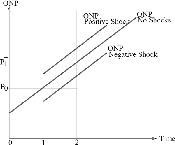
Crucially for the present paper, the effect on inflation of the economy-wide distribution of shocks depends on expected inflation. To see why, consider a firm which expects the (log) aggregate price level to rise steadily through time. With no shocks, this firm's optimal (log) output price also rises steadily as in Figure 4. Assume that the firm sets its output price at time 0 with the intention of re-setting it at time 2. Given this intention, it sets its output price initially at p_o, to minimise the difference between its actual and expected optimal price in the time interval between period-0 and period-2 (see Figure 4).^[7]

Now the firm's response to a shock at time 1, between regular price updates, depends on the sign, as well as the size, of the shock. A negative shock to its optimal price may not elicit a reaction because the firm knows that inflation will do much of the work of raising its optimal nominal price towards its current price p_o (see Figure 4). But after a positive shock of the same size, inflation raises its optimal nominal price further away from its current price p_o, and so the firm pays the menu cost and adjusts its price immediately up to p₁⁺.

Thus, with trend expected inflation, optimal pricing behaviour by firms generates economy-wide price adjustments that are asymmetric. Prices are “stickier” when a firm's optimal price falls than when it rises. Note, however, that it is the presence of trend expected inflation that generates the asymmetric price response. By contrast, when expected inflation is zero, the asymmetry disappears.

A corollary to this observation, which is central to this paper, is that there is a link between the dispersion (standard deviation) of economy-wide relative-price shocks and inflation when expected inflation is positive but not when it is zero. With trend expected inflation, few firms make special adjustments to their output prices in periods with a small dispersion of shocks. But in periods with a wide dispersion of shocks, many firms adjust their prices, and most of these adjustments are up. Hence, inflation rises above trend.^[8] By contrast, with zero expected inflation, a wide dispersion of shocks still causes many firms to adjust their prices, but as many adjust down as up. Then, a wide dispersion of shocks is not inflationary.

In the next section of the paper, we use industry-price data to test this key implication of the Ball-Mankiw model. Before doing so, however, there are a few issues to be addressed.

Firstly, as we have seen, the model predicts that a high dispersion of shocks is inflationary when expected inflation is positive but not when it is zero. In order to test this prediction with the data, however, it is necessary to know the model's prediction of the effect of dispersion on inflation over a range of rates of expected inflation from zero up to some relevant maximum rate.

Secondly, while the Ball-Mankiw model analyses the reaction of firms to shocks to their optimal prices, no data are available on the distribution of underlying shocks. All available data relate to the economy-wide distribution of industry price changes. From the perspective of the model, these data reveal only those shocks large enough to have induced a price response by firms. To compare with the data, we therefore derive model predictions for the relationship between the dispersion of industry price changes and inflation as a function of expected inflation.

3.2 Model Simulation Results

The model is sufficiently complex that we cannot derive closed-form expressions for the relationship between the dispersion of shocks and inflation. Instead, we present results derived from simulations of the model. These results are derived assuming all firms in an industry are identical so that shocks to the firms' optimal price (henceforth, optimal price shocks) are industry-specific. In any time-period, we assume the economy-wide distribution of optimal price shocks has a normal distribution N (0 ,SDS²) with the standard deviation of shocks, SDS, taking a (randomly chosen) value in the range . A period with a low economy-wide dispersion of shocks is one with , while a period with a high dispersion of shocks has .

We choose bounds for the dispersion of shocks, , to match features of the Australian data and assume all firms face identical menu costs. We also assume all firms face an identical distribution of possible shocks but, ex ante, are unaware whether the period will be one with a low or high economy-wide dispersion of shocks.

For given expected inflation, we choose a series of values of SDS in the range and, for each value of SDS, derive the inflation rate predicted by the model, Δp, and the value for SDP, the economy-wide standard deviation of industry price changes, generated by the model. For given expected inflation, these model simulations are usefully summarised by deriving coefficient estimates from two OLS regressions:^[9]

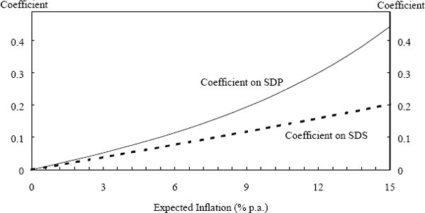
Figure 5 reports the results which are consistent with the intuitive arguments presented above. When expected inflation is zero, the model implies no relationship between the dispersion of shocks, SDS, and inflation, Δp, while with positive expected inflation, there is a positive relationship. Note also that as expected inflation rises, the model relationship between the dispersion of shocks and actual inflation becomes progressively stronger. Furthermore, as is clear from Figure 5, the same qualitative picture emerges when the regression is run with the standard deviation of industry price changes, SDP, replacing the standard deviation of shocks, SDS.^[10]

Before turning to empirical tests with industry price data, we address the implications of skewness in the distribution of underlying shocks. As Ball and Mankiw (1992b) stress, their model makes strong predictions about the impact on inflation of a skew distribution of underlying shocks. Again, this can be understood from a simple informal argument. If the economy-wide distribution of relative price shocks is positively skewed, there are big rises in the optimal price for a few industries offset by small falls in the optimal prices for the rest of the economy. Firms facing the big positive shocks adjust their prices up immediately, while the others make no special adjustment. It follows that a positively (negatively) skewed distribution of relative price shocks is inflationary (disinflationary) in the short-run. Furthermore, this argument clearly applies whatever the rate of expected inflation.

For our purposes, it is important to know how the presence of skewness in the distribution of shocks affects the links between dispersion, expected inflation and actual inflation. To address this issue, we again present results from a model simulation.^[11]

We make the same assumptions as before, with the exception that shocks are no longer normally distributed. Instead, we assume the economy-wide distribution of shocks is a sum of two normal distributions with different means and variances (suggested by the Australian data on industry price changes which often resemble the sum of two normal distributions, see Figure 2).^[12] Allowing the mean and/or variance of one of the two normal distributions to vary, implies that the dispersion and/or skewness of the underlying shocks also varies.

Parameters for the distribution of shocks are again chosen to match features of the Australian data, and the model results are now summarised by generating coefficient estimates from these two OLS regressions:

where Δp is again the model-generated aggregate inflation rate, SKS is the skewness of the economy-wide distribution of shocks and SKP is the skewness of the distribution of industry price changes.^[13]

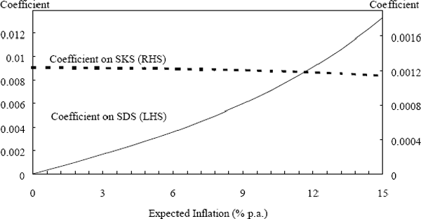
Results are shown in Figures 6 and 7. As the informal argument above should lead one to expect, the model implies that a rise in the skewness of shocks, SKS, is always inflationary (Figure 6). Furthermore, the effect of the skewness of shocks on inflation is largely independent of the rate of expected inflation. Interestingly, the effect of expected inflation on the link between the dispersion of shocks, SDS, and the inflation rate is the same (qualitatively) as its effect in the earlier simulation when skewness played no role. That is, a rise in the rate of expected inflation progressively increases the strength of the link between dispersion and actual inflation whether the underlying shocks are symmetric or not.

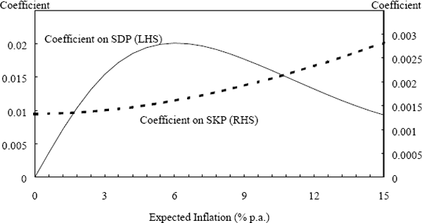
Again, the story is fairly similar when the moments of industry price changes, SDP and SKP, replace the moments of shocks, SDS and SKS, in the inflation regression (Figure 7). The coefficient on SKP is relatively insensitive to expected inflation, while the coefficient on SDP rises strongly with expected inflation (at least up to expected inflation of about 6% per annum).^[14]

To summarise, the Ball-Mankiw model has a rich set of implications for the links between expected inflation, the economy-wide distribution of relative-price shocks and actual inflation. When expected inflation is very low, a rise in the dispersion of shocks has minimal impact on actual inflation while a rise in the skewness of shocks is inflationary. When expected inflation is higher, a rise in either dispersion or skewness is inflationary. Furthermore, these statements remain true when the (economy-wide) moments of industry price changes replace the moments of the underlying shocks.

Before turning to empirical tests, we briefly touch on the relevance of the Ball-Mankiw model for the statistical test in the earlier section: Are price falls special? As we have discussed, the Ball-Mankiw model predicts that in the presence of expected trend inflation, prices are more sticky when falling than when rising. It follows that, with expected trend inflation, the proportion of price falls should be less than the proportion of price rises greater than twice the inflation rate. However, if the economy-wide distribution of price shocks is often negatively skewed ex post, this argument is not very critical because in these periods, the Ball-Mankiw model predicts that the proportion of price falls will be higher than the proportion of price rises greater than twice the inflation rate. The fact that the statistical tests reported in the earlier section accept the hypothesis that the proportions are equal is therefore corroborative evidence that the underlying shocks are often significantly negatively skewed.

Footnotes

In this section, we use informal arguments to derive the model's key implications, while a formal summary of it is provided in Appendix 2. [6]

For ease of exposition, we assume the whole time interval between periods 0 and 2 is relevant to the initial pricing decision. In fact, the formal model is set in discrete time (Appendix 2). [7]

Firms are forward-looking and know the distribution of possible shocks, though, ex ante, they are unaware whether the period will be one with a low or high economy-wide dispersion of shocks. These assumptions imply that inflation falls below trend in periods with a low dispersion of shocks and rises above trend when the dispersion of shocks is high. By assumption, deviations from trend inflation do not change future expected inflation (that is, shocks to the aggregate price level are permanent.) [8]

The period of the model is assumed to be six months. For given expected inflation, model results are derived for ten values of SDS in the range , which leads to ten different values for SDP and for Δp. The regression results are derived from these ten simulated outcomes. Both regressions provide very good empirical descriptions of inflation in the model, with R² > 0.94 for all values of expected inflation up to an annualised rate of 15% p.a. See Appendix 2 for further technical details. [9]

How large is the predicted effect on inflation? With expected inflation of zero, of course, any change in the economy-wide dispersion of shocks has no impact on actual inflation. With expected inflation of 3% p.a., a two standard deviation rise in the dispersion of shocks leads to a rise in actual inflation of 0.5% p.a. (measured at an annualised rate) while with expected inflation of 8% p.a., the rise in actual inflation is a much larger 1.2% p.a. (Recall that the model is calibrated to match actual Australian data.) Thus, with expected inflation of 8% p.a., a typical rise in the economy-wide dispersion of shocks from one six-month period to the next is predicted to lead to a substantial, albeit temporary, rise in inflation. [10]

Ball and Mankiw (1992b) also present model simulation results for the relationship between dispersion and skewness of industry price changes and inflation, but their results are restricted to the case when expected inflation is zero. [11]

The US distribution of price changes often looks the same – see Figure 3 in Ball and Mankiw (1992b). While the distribution of price changes is not the same as the distribution of shocks, the former at least provides a guide for the latter. [12]

As before, both regressions provide very good empirical descriptions of inflation in the model, with R² > 0.9 for all values of expected inflation up to 15% p.a. [13]

We also established that the moments of industry price changes are well explained by the respective moments of underlying shocks. For the regression, SDP =α + β SDS+ u , R² > 0 96 for all rates of expected inflation up to 15% p.a., while for the regression, SK P =α + β SK S+ u, R² > 0.88. [14]